5  The First City

What is the minimum community that can sustain itself?

Not a single cell – we established that in the last chapter. One organism, one metabolism, and the waste piles up until the system chokes. You need at least two metabolic strategies to close even the simplest biogeochemical cycle. But two is also not enough, because real environments have more than one energy source and more than one waste product. So: what is the minimum?

The answer, preserved in rocks 3.5 billion years old and still visible today in Shark Bay, Australia, is a bacterial mat.¹ A few millimeters thick, slippery, unremarkable to the eye. Green on top. Pink beneath. Dark below. Three layers, three metabolic guilds, and a nearly closed material cycle that required no external input beyond sunlight and seawater.

Bacterial mats were the dominant expression of life on this planet for over two billion years.² They were not a rough draft. They were the dominant form of life for their era: self-sustaining communities so stable that the basic design persisted from the Archean into the Proterozoic and, in diminished form, persists today. They built the stromatolites whose layered fossils record one of the longest continuous biological records on Earth.³ They invented metabolic partnerships that would later be repurposed inside the cells of every plant and animal alive. And they did all this without a nucleus, without organelles, without anything you’d recognize as coordination – just chemistry, gradients, and the relentless pressure of thermodynamics selecting for communities that could close their own loops.

5.1 Three neighborhoods

A bacterial mat is not a uniform film. It is layered, and the layering is not accidental – it is imposed by physics. Light attenuates with depth. Chemical gradients steepen. Each layer creates the boundary conditions for the layer below it, the way a city’s infrastructure determines what can be built on each block.

The analogy to a city is more than decorative. A city works because different neighborhoods specialize: one district generates power, another processes waste, a third manufactures goods. The neighborhoods depend on each other. Remove one and the others degrade. A bacterial mat operates on the same principle, except the “districts” are defined by wavelength, chemistry, and metabolic strategy rather than zoning laws.

[FIGURE: Cross-section of an idealized bacterial mat, drawn to scale (~5 mm thick). Four layers are shaded: (1) green canopy at top – anoxygenic phototrophs using H2S, labeled with “visible light in, organic carbon out”; (2) pink layer below – purple bacteria using longer wavelengths; (3) pale layer – heterotrophs and fermenters, consuming dead organic matter; (4) dark layer at bottom – sulfate reducers, converting sulfate back to H2S. Arrows show the sulfur cycle closing: H2S rises from bottom, is oxidized at top, sulfate sinks back down. Caption: “Four metabolisms, one closed loop. The mat recycles its own waste.”]

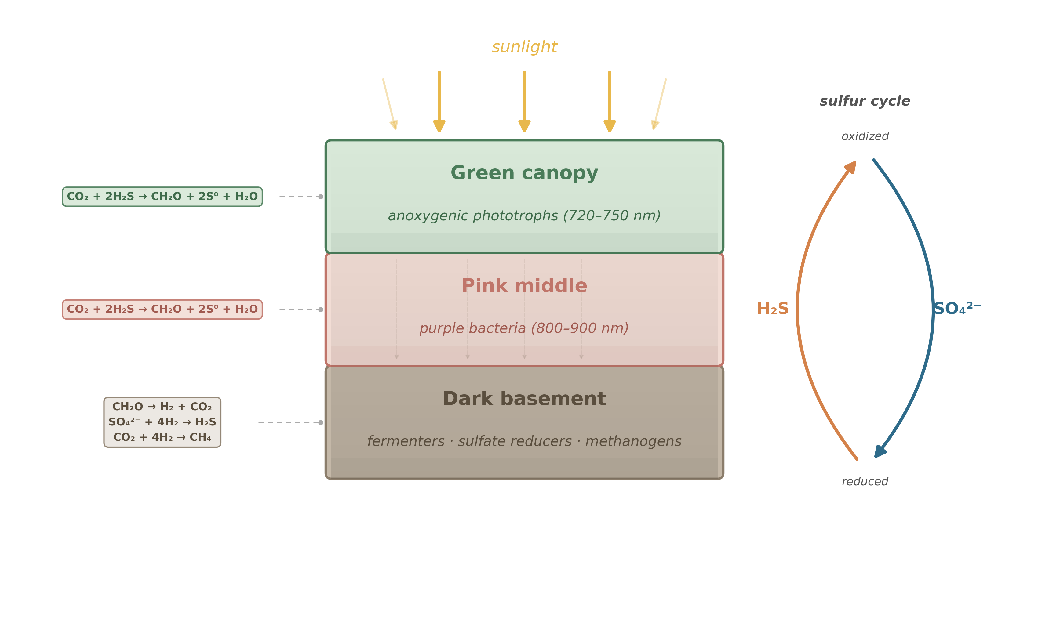
5.1.1 The green canopy

The top layer is green, and the green is functional. Here live anoxygenic photosynthetic bacteria – ancestors of the cyanobacteria that would later learn the far more aggressive trick of splitting water. But we are still in the early Archean, and that revolution is hundreds of millions of years away.⁴

These surface-dwellers harvest sunlight across the visible spectrum, but their electron source is not water. It is hydrogen sulfide, H\(_2\)S – the same gas that gives rotten eggs their smell.⁵ The overall logic is straightforward: capture photons, use their energy to strip electrons from H\(_2\)S, and feed those electrons into carbon fixation. The waste products are elemental sulfur or sulfate, depending on the species and conditions.

This is a good deal, thermodynamically. Sunlight provides abundant energy, and H\(_2\)S is plentiful in the anoxic early ocean, venting from hydrothermal systems and recycled from deeper in the mat itself. The top layer is the city’s power plant: it captures the primary energy input and converts it into organic carbon that the rest of the community will eventually consume.

But there is a constraint that matters. The green layer absorbs the short-wavelength, high-energy photons – the blues and greens. By doing so, it casts a shadow. Not total darkness, but a filtered light, depleted in the wavelengths the top layer already harvested. Whatever lives below must make do with what passes through.

5.1.2 The pink middle

Below the green canopy, the light is different. The short wavelengths are largely gone, absorbed or scattered by the layer above. What remains is longer-wavelength light – reds and near-infrared – and it is in this filtered glow that the second layer thrives.

These are alpha-proteobacteria, ancestors of the purple bacteria that still inhabit microbial mats today.⁶ They carry different photosynthetic pigments, tuned to the wavelengths the green layer rejected. This is not coincidence; it is niche partitioning driven by the physics of light absorption.⁷ If you tried to put another green-pigmented organism here, it would starve – the photons it needs are already consumed. The pink layer survives precisely because it uses a different part of the spectrum.

The metabolic logic is similar to the top layer: capture photons, fix carbon, grow. But the energy input per photon is smaller (longer wavelength means lower energy per photon), and the flux is reduced. The pink layer operates on thinner margins. It is the city’s secondary industry – still productive, but working with what the primary sector leaves behind.

This arrangement – spectral stratification dictated by pigment absorption – is one of the oldest examples of resource partitioning in the history of life.⁸ It works because physics makes different wavelengths available at different depths, and evolution filled each niche with organisms tuned to exploit whatever light remained. The principle is the same one that structures a forest canopy, except the “trees” here are single cells and the “forest” is a few millimeters tall.

5.1.3 The dark basement

Below the pink layer, the light is effectively gone. Whatever survives here must live without photons entirely. This is the mat’s basement – its recycling district – and it runs on chemistry alone.

Several guilds coexist in this dark zone, and their interactions form the critical loop that makes the whole community self-sustaining.

Fermenters break down the organic matter that rains from above – dead cells, exudates, structural polymers. Fermentation does not require an external electron acceptor; it reshuffles the carbon and hydrogen within organic molecules, producing a mix of small organic acids, alcohols, CO\(_2\), and molecular hydrogen (H\(_2\)). The energy yield per molecule is modest, but the substrates are abundant.

Sulfate reducers pick up where the fermenters leave off.⁹ They use the H\(_2\) that fermentation produces as an electron donor and reduce the sulfate (SO\(_4^{2-}\)) that was generated as waste by the photosynthetic top layer, converting it back to hydrogen sulfide:

\[ 4\,\text{H}_2 + \text{SO}_4^{2-} + 2\,\text{H}^+ \longrightarrow \text{H}_2\text{S} + 4\,\text{H}_2\text{O} \]

Read that equation carefully. The sulfate reducers are completing a cycle: the top layer oxidized H\(_2\)S to sulfate; the bottom layer reduces sulfate back to H\(_2\)S. The “fuel” for the top layer is regenerated in the basement. The city recycles its own waste into raw material.

Methanogens run a parallel operation. They too consume the H\(_2\) from fermentation, but instead of reducing sulfate, they reduce CO\(_2\) to methane:

\[ 4\,\text{H}_2 + \text{CO}_2 \longrightarrow \text{CH}_4 + 2\,\text{H}_2\text{O} \]

Methanogens and sulfate reducers compete for the same electron donor – H\(_2\) – and the outcome of that competition depends on local concentrations and thermodynamics.¹⁰ Where sulfate is abundant, sulfate reducers tend to win (their reaction yields more energy per mole of H\(_2\)). Where sulfate is scarce, methanogens dominate. This is an early example of a principle we will formalize later: the redox ladder is not a rigid law, but a tendency shaped by local supply.

Methanogens today live almost everywhere that lacks oxygen and has fermenters to supply them – in wetland sediments, in rice paddies, in landfills, and in the intestines of animals, including ours.¹¹ Their persistence across such different environments is a testament to how general and robust the methanogenic niche is. If there is organic carbon and no strong oxidant, someone will eventually make methane.

5.2 The beauty of the closed cycle

Step back and look at the whole mat as a single system. What you see is a community that has nearly closed its own material loops.

The top layer fixes CO\(_2\) into organic carbon using sunlight and H\(_2\)S. It releases sulfate as waste. The middle layer does the same at longer wavelengths, adding to the pool of organic matter. The bottom layer ferments the organic matter, producing H\(_2\) and small molecules. Sulfate reducers use that H\(_2\) to convert sulfate back to H\(_2\)S – which rises back to the top layer as fuel. Methanogens convert CO\(_2\) to methane, some of which escapes, some of which is oxidized anaerobically if the right partners are present.

The only net inputs the community needs are sunlight and whatever dissolved gases and minerals the ocean provides. The only net outputs are heat (entropy export, as Chapter 1 described) and whatever metabolic byproducts escape into the water column.

This is why the design was so stable. A community that recycles its own key substrates is buffered against fluctuations in external supply. If the ocean delivers less H\(_2\)S from hydrothermal vents, the mat’s internal sulfur cycle can partially compensate. If organic carbon accumulates too fast for the fermenters, the surplus gets buried and incorporated into the growing stromatolite structure.

The community was quite stable in this form and could persist for hundreds of millions of years.¹² Not because individual cells were immortal, but because the architecture was self-reinforcing. Each metabolic guild created the conditions that sustained the others. Remove the fermenters and the sulfate reducers starve for H\(_2\). Remove the sulfate reducers and the top layer runs out of H\(_2\)S. Remove the phototrophs and the entire carbon and energy input disappears. The community is the ecosystem.

5.3 Stromatolites: the fossil cities

If bacterial mats were the living cities, stromatolites are their ruins.

A stromatolite is a layered rock structure, often dome-shaped or columnar, built by the gradual accumulation of mineral and organic layers.¹³ The mechanism is simple in principle: the mat grows on a surface, trapping and binding sediment grains. Calcium carbonate precipitates from the surrounding water – partly through abiotic chemistry (CO\(_2\) consumption during photosynthesis shifts the local carbonate equilibrium), partly through direct microbial activity. A thin mineral crust forms over the living mat. The mat grows upward through the crust, re-establishing itself at the surface. Another layer of sediment and mineral accumulates. Repeat for millions of years.

The result is a laminated structure that records the rhythm of growth – sometimes seasonal, sometimes driven by other environmental cycles. The oldest convincing stromatolites date to about 3.5 billion years ago, from the Pilbara region of Western Australia and the Barberton Greenstone Belt in South Africa.¹⁴ Whether the very oldest structures are truly biological or purely chemical remains debated, but by 3.0 billion years ago the evidence is strong: these layered formations carry isotopic and structural signatures that are difficult to explain without biology.¹⁵

You can still visit living stromatolites today. In Shark Bay, Western Australia, hypersaline conditions exclude the grazing animals that would otherwise eat microbial mats, and stromatolites grow in shallow pools much as they might have in the Archean.¹⁶ They are not relics in the museum sense – they are working communities, still running the same basic metabolic architecture, still layered, still cycling sulfur and carbon internally.

The difference is context. In the Archean, bacterial mats and their stromatolite constructions were the only game in town. They dominated every shallow-water environment on the planet. Today they survive only in ecological refuges where competition and predation are reduced. The design hasn’t failed; it has been outcompeted in most habitats by the organisms that its own metabolic innovations eventually made possible.

5.4 Reading the isotopes: fingerprints of ancient metabolism

How do we know these communities were autotrophic – that they were fixing carbon from CO\(_2\) rather than simply rearranging pre-existing organic molecules?

The answer is written in carbon isotopes. Carbon has two stable isotopes: ¹²C (six protons, six neutrons) and ¹³C (six protons, seven neutrons). The heavier isotope behaves slightly differently in chemical reactions – it forms slightly stronger bonds, reacts slightly more slowly, and is slightly less likely to be incorporated into products during enzymatic reactions.

The enzyme that matters most here is RuBisCO – ribulose-1,5-bisphosphate carboxylase/oxygenase – the enzyme responsible for the first step of the Calvin cycle, where CO\(_2\) is fixed into organic carbon.¹⁷ RuBisCO has a measurable preference for ¹²C over ¹³C. When it grabs a CO\(_2\) molecule from the environment, it is slightly more likely to grab the lighter isotope.¹⁸ The result: organic carbon produced by autotrophs is enriched in ¹²C relative to the CO\(_2\) they consumed.

This isotopic fingerprint survives geological time. In Greenland, graphite inclusions within apatite crystals dated to 3.8 billion years ago show a carbon isotope ratio shifted toward light carbon – the signature of autotrophic carbon fixation.¹⁹ The organisms that made this carbon are long gone, but their isotopic preferences are preserved in rock.

A similar story plays out with nitrogen. The enzyme nitrogenase, which fixes atmospheric N\(_2\) into biologically usable ammonia (NH\(_3\)), also discriminates between isotopes.²⁰ Together, RuBisCO and nitrogenase are the key enzymes by which inorganic substances enter the biosphere – the gatekeepers between the mineral world and the living one.

The quantitative framework for isotope fractionation – the \(\delta^{13}\)C scale, its measurement, and its limitations as a biosignature – is detailed in Appendix A.

5.5 Microbes as geological agents

Microbial mats did not merely inhabit the early Earth – they reshaped it. Photosynthesis raises local pH and drives carbonate precipitation; sulfate reduction generates sulfide minerals; iron-oxidizing bacteria leave behind iron oxides. The sedimentary rock record is, to a remarkable degree, a record of microbial metabolism.²¹ The relationship between life and geology is bidirectional: the planet shaped the first communities, and those communities shaped the planet back.

5.6 The first metabolisms

The earliest metabolisms were likely chemoautotrophic. Phylogenetic reconstruction places methanogenesis – CO\(_2\) + 4 H\(_2\) \(\rightarrow\) CH\(_4\) + 2 H\(_2\)O – among the most ancient archaeal metabolisms, though its exact position in the tree remains debated.²² Both substrates were abundant on the early Earth, produced abiotically by volcanic outgassing and water-rock reactions. No light required. No complex organic substrates. Just two simple gases and enzymes sophisticated enough to catalyze the reaction at biologically useful rates.

5.7 The speed limit of life: why enzymes matter

We have been describing metabolisms – reactions that microbes catalyze to earn a living. But there is a question we have deferred since Chapter 1: why do these reactions need catalysis at all?

The thermodynamic answer is clear enough. Many of the reactions that life depends on are spontaneous – they have negative \(\Delta G\) under environmental conditions. Hydrogen and CO\(_2\) “want” to become methane in the same way that a ball at the top of a hill “wants” to roll down. The free energy is there.

But spontaneity says nothing about speed. A reaction can be thermodynamically favorable and yet proceed so slowly that it might as well not happen. Methane formation from CO\(_2\) and H\(_2\) at room temperature, without a catalyst, would take longer than the age of the universe to produce a detectable quantity.²³ The energy is available. The rate is not.

This is why enzymes exist. They are the difference between a reaction that is possible in principle and a reaction that is fast enough to sustain a living cell.

5.8 What enzymes actually do

Enzymes are protein catalysts that accelerate specific chemical reactions by factors of 10\(^8\) to 10\(^{17}\) without being consumed.²⁴ Three properties define them: they are needed in small amounts (one molecule can process thousands of substrates per second); they emerge from each reaction cycle unchanged; and they have no effect on thermodynamics – an enzyme cannot make an unfavorable reaction favorable, it can only speed the approach to equilibrium.

That last point matters. Enzymes do not push reactions in one direction. They accelerate both forward and reverse reactions equally. The net direction is still dictated by \(\Delta G\). The enzyme just ensures that the system reaches its thermodynamic destiny faster.

Catalysis happens at the active site – a pocket whose shape and charge complement the substrate. The enzyme accelerates the reaction by orienting reactive groups, stabilizing the transition state electrostatically, and in some cases physically straining the bonds that need to break. Many enzymes also require cofactors – metal ions (iron, zinc, molybdenum) or organic molecules (NAD\(^+\), FAD, coenzyme A) that participate directly in catalysis. The deep dependence of modern biochemistry on iron cofactors is likely a molecular fossil of life’s origin in an iron-rich, anoxic ocean. The details of active-site mechanisms, cofactor roles, and inhibition types are in Appendix A.

5.9 Michaelis-Menten kinetics: the speed limit

The rate at which an enzyme works depends on substrate supply. Michaelis and Menten (1913) formalized the relationship:²⁵ \(V = V_{\max}[\text{S}]/([\text{S}] + K_m)\), where \(V_{\max}\) is the maximum rate at full saturation and \(K_m\) is the substrate concentration at which the rate is half-maximal.

At low substrate (\([\text{S}] \ll K_m\)), the rate scales linearly with supply – the enzyme has idle time between encounters. At high substrate (\([\text{S}] \gg K_m\)), the rate plateaus at \(V_{\max}\) – every enzyme molecule is busy. In a bacterial mat, substrate concentrations are set not by a lab technician but by the balance between production, consumption, and diffusion. An enzyme with \(K_m\) below the local substrate concentration runs near \(V_{\max}\); one with \(K_m\) above it tracks every fluctuation in supply.

This hyperbolic curve is the speed limit of life. Metabolism is never infinitely fast, even when energy is abundant. Appendix A covers the Lineweaver-Burk graphical method, enzyme inhibition types, and temperature/pH dependencies.

5.10 The mat as a metabolic circuit

Now we can put the pieces together. The bacterial mat is not just a community of organisms sharing space. It is a metabolic circuit – a system in which the waste of each guild becomes the substrate of another, and the kinetics of each enzyme determines the rate at which that handoff occurs.

The phototrophs at the top fix carbon at a rate governed by light intensity and their carbon-fixation enzymes (including, eventually, RuBisCO). The fermenters in the dark layer process the organic carbon at rates governed by their hydrolytic and fermentative enzymes. The sulfate reducers consume H\(_2\) at rates dictated by their hydrogenases and dissimilatory sulfite reductases. And the methanogens compete for the same H\(_2\) using their own enzymatic machinery.

At every step, Michaelis-Menten kinetics applies. At every step, the rate depends on local substrate concentration, which depends on the rates of the reactions that produce that substrate, which depend on their substrate concentrations, and so on. The entire mat is a system of coupled hyperbolas – each enzyme’s rate feeding into the next enzyme’s supply.

This is why the mat can be stable for hundreds of millions of years. It is a system of feedback loops. If the top layer produces more organic matter than the fermenters can process, organic carbon accumulates, fermentation rates increase (moving rightward along the Michaelis-Menten curve), and the excess is eventually consumed. If sulfate becomes scarce, sulfate reduction slows, H\(_2\) accumulates, and methanogens gain an advantage. The system self-regulates – not through any central control, but through the thermodynamics and kinetics of coupled chemical reactions.

Notice what the mat is not doing. It is not optimizing. No guild is maximizing its growth rate, its energy yield, or its share of the electron budget. Each guild is running the reactions its enzymes can catalyze, at rates set by local substrate concentrations, and the steady state that emerges is a consequence of constraints – not a solution to any optimization problem. The mat satisfices. It finds a configuration that covers every guild’s maintenance costs and happens to close the material loops, not because the community “wants” to close them, but because any configuration that fails to recycle a key substrate eventually starves the guild that depends on it and collapses.

This matters for modeling. If you assume optimization – that sulfate reducers outcompete methanogens everywhere sulfate is present, that redox zones are sharp, that one reaction dominates per depth interval – you get a model that is elegant and wrong. Real mats show overlap, coexistence, and zones where “losing” reactions persist at low rates. The satisficing view explains this: organisms do not compete to extinction when both can cover their costs. They coexist in the fuzzy margin where \(\Delta G\) is negative for both, and the boundary between them is not a line but a gradient.

5.11 What we sacrificed

A word about what we have simplified.

The three-layer model described in this chapter is a useful idealization, but real bacterial mats are messier. Gradients are not sharp boundaries; they are continuous. Species are not neatly confined to one layer; many are motile and migrate with the light cycle. The chemistry is not limited to sulfur and carbon; nitrogen, phosphorus, iron, and trace metals all play roles that we have omitted here.

We also treated enzymes as isolated catalysts following simple Michaelis-Menten kinetics. In reality, enzymes inside cells are organized into pathways and complexes, subject to allosteric regulation, product inhibition, and competition for shared cofactors. The Michaelis-Menten equation describes one enzyme acting on one substrate in a well-mixed solution. Inside a cell – let alone inside a millimeter-thick mat with steep gradients – the conditions for that equation are only approximately met.

These simplifications are not errors. They are deliberate trades: we sacrifice realism for a framework that can be interrogated quantitatively. The Michaelis-Menten curve, the closed sulfur cycle, the three-layered architecture – these are models, not photographs. Their value is that they let you ask, “What would change if I doubled the sulfate supply?” or “What happens to the mat if light intensity drops?” and get a directional answer. We will build on them, adding complexity where it earns its keep.

5.12 Takeaway

• Bacterial mats were the dominant life form on Earth for over two billion years: layered, self-sustaining communities with closed material cycles.
• The three-layer architecture (phototrophs, secondary phototrophs, dark-zone recyclers) was dictated by physics – light attenuation, chemical gradients, and thermodynamic competition.
• Stromatolites are the fossil record of these communities, preserved in layered carbonate structures dating to 3.5 billion years ago.
• Carbon isotope fractionation by RuBisCO provides a durable biosignature, detectable in rocks 3.8 billion years old.
• Enzymes accelerate reactions by 10\(^8\) to 10\(^{17}\)-fold; Michaelis-Menten kinetics (\(V = V_{\max}[\text{S}]/([\text{S}] + K_m)\)) describes the speed-versus-supply tradeoff governing every metabolic reaction in the mat.
• The mat satisfices: it finds a steady state dictated by constraints, not optimization. Competing metabolisms coexist wherever both can cover maintenance costs.

---

1. Living stromatolites in Shark Bay, Western Australia, provide modern analogs of ancient mat communities. The hypersaline conditions exclude grazing metazoans that would otherwise consume the mats. See David J. Des Marais, “Biogeochemistry of Hypersaline Microbial Mats Illustrates the Dynamics of Modern Microbial Ecosystems and the Early Evolution of the Biosphere,” Biological Bulletin 204 (2003): 160–167. (Des Marais 2003)

2. Bacterial mats were the dominant form of life from at least 3.5 billion years ago through much of the Proterozoic (ending ~540 million years ago), a span exceeding 2 billion years. See David J. Des Marais, “Microbial Mats and the Early Evolution of Life,” Trends in Ecology and Evolution 5 (1990): 140–144. (Des Marais 1990)

3. Stromatolites provide one of the longest continuous records of biological activity on Earth, with morphological and geochemical signatures spanning from the Archean to the present. See J. William Schopf, “Fossil Evidence of Archaean Life,” Philosophical Transactions of the Royal Society B 361 (2006): 869–885. (Schopf 2006)

4. Anoxygenic photosynthesis (using electron donors such as H\(_2\)S, Fe\(^{2+}\), or H\(_2\) rather than water) predates oxygenic photosynthesis. Robert E. Blankenship, “Early Evolution of Photosynthesis,” Plant Physiology 154 (2010): 434–438. (Blankenship 2010)

5. Green sulfur bacteria (Chlorobiaceae) and purple sulfur bacteria (Chromatiaceae) oxidize hydrogen sulfide during anoxygenic photosynthesis, depositing elemental sulfur either externally or internally depending on the lineage. See Alexandr Markov, Birth of Complexity: Evolutionary Biology Today (2010). (Markov 2010)

6. Purple bacteria, including members of the Proteobacteria, use bacteriochlorophylls with absorption maxima in the near-infrared (800–900 nm), allowing them to harvest light at wavelengths not absorbed by overlying green-pigmented phototrophs. (Markov 2010)

7. Spectral niche partitioning in microbial mats is driven by the wavelength-dependent attenuation of light through successive photosynthetic layers. Each layer absorbs photons matching its pigment absorption spectra, creating distinct light environments at different depths. See David J. Des Marais, “Microbial Mats and the Early Evolution of Life” (1990). (Des Marais 1990)

8. Resource partitioning by wavelength was likely one of the earliest forms of ecological niche differentiation, allowing multiple photosynthetic guilds to coexist within millimeters of vertical space. This principle operates in modern microbial mats and was likely present in Archean mat communities. (Des Marais 2003)

9. Sulfate reduction is thermodynamically favorable under anoxic conditions and is catalyzed by dissimilatory sulfate reducers. Bo Barker Jørgensen, “Mineralization of Organic Matter in the Sea Bed—the Role of Sulphate Reduction,” Nature 296 (1982): 643–645. (Jørgensen 1982)

10. The competition between sulfate reducers and methanogens for H\(_2\) is determined by the Gibbs free energy yields of the respective reactions under local conditions. Sulfate reduction yields more energy per mole of H\(_2\) oxidized, giving sulfate reducers a thermodynamic advantage where sulfate is available. See Rudolf K. Thauer et al., “Energy Conservation in Chemotrophic Anaerobic Bacteria,” Bacteriological Reviews 41 (1977): 809. (Thauer et al. 1977)

11. Methanogens (domain Archaea) inhabit diverse anoxic environments including sediments, wetlands, animal digestive tracts, and deep subsurface habitats. Their metabolic versatility and reliance on simple substrates (H\(_2\)/CO\(_2\), acetate, methylated compounds) make them globally distributed. (Thauer et al. 1977)

12. The architectural stability of bacterial mat communities arises from metabolic interdependence: each guild generates substrates or removes wastes for others, creating self-reinforcing feedback loops. See Alexandr Markov, Birth of Complexity (2010). (Markov 2010)

13. Stromatolite formation involves microbial trapping and binding of sediment particles combined with precipitation of calcium carbonate, often induced by photosynthetic CO\(_2\) consumption that raises local pH and shifts carbonate equilibrium. (Des Marais 2003)

14. The oldest widely accepted stromatolites are from the ~3.48 Ga Dresser Formation (Pilbara, Western Australia). Abigail C. Allwood et al., “Stromatolite Reef from the Early Archaean Era of Australia,” Nature 441 (2006): 714–718. (Allwood et al. 2006)

15. Biosignatures in ancient stromatolites include lamination patterns consistent with photosynthetic growth cycles, carbon isotope fractionation indicative of autotrophy, and morphologies difficult to produce abiotically. (Schopf 2006)

16. Modern stromatolites in Shark Bay’s Hamelin Pool demonstrate that microbial mat communities can build carbonate structures under conditions analogous to those of the Precambrian, when grazing metazoans were absent or rare. (Des Marais 2003)

17. RuBisCO (ribulose-1,5-bisphosphate carboxylase/oxygenase) catalyzes the carboxylation of ribulose-1,5-bisphosphate, the first committed step of the Calvin-Benson-Bassham cycle. It is the most abundant enzyme on Earth. See Gerald Karp, Cell and Molecular Biology: Concepts and Experiments, 7th ed. (2008). (Karp 2008)

18. Enzymatic carbon isotope fractionation during autotrophic CO\(_2\) fixation produces organic matter depleted in ¹³C by ~20–30 per mil relative to source CO\(_2\). Graham D. Farquhar et al., “Carbon Isotope Discrimination and Photosynthesis,” Annual Review of Plant Physiology and Plant Molecular Biology 40 (1989): 503–537. (Farquhar, Ehleringer, and Hubick 1989)

19. Graphite inclusions in 3.8 Ga apatite from the Isua supracrustal belt (Greenland) show ¹³C depletion consistent with biological carbon fixation, providing the oldest putative isotopic biosignature. Manfred Schidlowski, “A 3,800-Million-Year Isotopic Record of Life from Carbon in Sedimentary Rocks,” Nature (1988). (Schidlowski 1988)

20. Nitrogenase catalyzes the reduction of atmospheric N\(_2\) to NH\(_3\), the only biological pathway for nitrogen fixation. The enzyme also fractionates nitrogen isotopes, preferentially incorporating ¹⁴N. James B. Howard and Douglas C. Rees, “Structural Basis of Biological Nitrogen Fixation,” Chemical Reviews 96 (1996): 2965–2982. (Howard and Rees 1996)

21. Microbial metabolism drives mineral precipitation, dissolution, and transformation. Photosynthesis alters pH and carbonate chemistry; sulfate reduction generates sulfide minerals; iron oxidation produces iron oxides. John W. Moreau et al., “Extracellular Proteins Limit the Dispersal of Biogenic Nanoparticles,” Science 316 (2006): 1600–1603. (Moreau et al. 2006)

22. Methanogenesis is phylogenetically deep within the Archaea, suggesting it is among the most ancient metabolisms. Eric Bapteste et al., “Higher-Level Classification of the Archaea: Evolution of Methanogenesis and Methanogens,” Archaea 1 (2005): 353–363. (Bapteste, Brochier, and Boucher 2005)

23. Uncatalyzed biochemical reactions can have half-lives ranging from seconds to billions of years. Without enzymes, reactions essential for life (e.g., peptide bond hydrolysis, phosphate ester cleavage) would proceed far too slowly to sustain metabolism. Richard Wolfenden and Mark J. Snider, “The Depth of Chemical Time and the Power of Enzymes as Catalysts,” Accounts of Chemical Research 34 (2001): 938–945. (Wolfenden and Snider 2001)

24. Enzymes accelerate reaction rates by factors typically ranging from 10\(^8\) to 10\(^{17}\), with some enzymes (e.g., orotidine 5’-monophosphate decarboxylase) achieving rate enhancements exceeding 10\(^{23}\). Gerald Karp, Cell and Molecular Biology (2008). (Karp 2008)

25. Leonor Michaelis and Maud L. Menten, “Die Kinetik der Invertinwirkung,” Biochemische Zeitschrift 49 (1913): 333–369. The Michaelis-Menten equation describes enzyme kinetics under steady-state assumptions. (Michaelis and Menten 1913)