10 Cities Without Sunlight
Somewhere in the Earth’s crust, a cell divides once per century. Its energy source is hydrogen gas, produced by the radioactive decay of uranium in the surrounding rock. Its electron acceptor is sulfate, trapped in mineral inclusions since the Archean. No photon has reached it in millions of years. It has no genes for oxygen use, almost no genes for oxygen defense. By every measure that laboratory microbiologists use to define “alive,” it barely qualifies – and yet it persists, and it reproduces, on a timescale measured in centuries.
The organism is Candidatus Desulforudis audaxviator. It was discovered in 2006, when a drilling crew at the Mponeng gold mine in South Africa punched through rock at 2.8 kilometers below the surface and hit water.
The water was hot – slightly above 60 degrees Celsius – alkaline, and saturated with a cocktail of dissolved chemicals: sulfate, molecular hydrogen, methane, carbon dioxide, and a scattering of simple organic molecules like formate and acetate. The rock enclosing it was basalt, part of a formation 2.7 billion years old. The water had been sealed down there for millions of years, in the dark, under crushing pressure, with no connection to the surface.
And it was alive.
Not teeming – not a jungle. But when Li-Hung Lin and colleagues analyzed the microbial community in that fracture water, they found something startling: a functioning ecosystem, dominated by a single bacterial species, running on chemistry that the rock itself provided.1 Most of the organic matter in the water had an abiogenic origin – produced not by photosynthesis or any biological process, but by geological reactions between water and minerals deep in the crust. The hydrogen came from radiolysis of water by uranium decay in the surrounding rock. The sulfate came from ancient seawater trapped in mineral inclusions.
Life, in this place, was not borrowing from the sun. It was borrowing from the Earth’s interior.
10.1 The brave wanderer
The organism that dominated that fracture water – comprising over 99.9 percent of the community – received one of the more literary names in microbiology: Candidatus Desulforudis audaxviator. The name comes from a Latin phrase in Jules Verne’s Journey to the Center of the Earth: “Descende, audax viator, et terrestre centrum attinges” – “Descend, brave traveler, and you will reach the center of the Earth”.2
The name was earned. When Dylan Chivian and colleagues reconstructed the organism’s genome from metagenomic data, they found a cell equipped for remarkable self-sufficiency. D. audaxviator carries a complete genetic toolkit for life in extreme isolation: it fixes its own carbon from CO\(_2\), fixes atmospheric nitrogen (there is no “atmosphere” down there, but trace dissolved N\(_2\) suffices), and harvests energy by reducing sulfate with molecular hydrogen. Thermodynamic calculations confirm that under the conditions of the Mponeng fracture water – the specific concentrations of H\(_2\), sulfate, and products present – this metabolism is the most energetically favorable option available.3 The calculated Gibbs energy yield is just barely sufficient to support ATP synthesis, placing this organism at the thermodynamic edge of life.4
What the genome does not contain is equally telling. There are zero genes for oxygen use. Minimal genes for oxygen defense – a lone superoxide dismutase but no catalase, no peroxidase, little of the protective machinery that aerobic or even facultatively anaerobic organisms carry as insurance. This organism has not dealt with oxygen for a very long time.5
Alongside D. audaxviator, the community includes roughly 25 other species, among them four methanogenic archaea. But the brave wanderer is the keystone – the organism that, more than any other, demonstrates how little a cell needs from its environment to persist for geological time. Lin and colleagues called it “the first proven case of autonomous long existence of living organisms in the bowels of the earth, without any connection with the big biosphere”.6
The fracture water community made its journey underground millions of years ago – noble gas dating suggests residence times of 3 to 25 million years, depending on the fracture system. Since then, it has survived on the thin trickle of chemical energy that radioactive decay and water-rock reactions provide. No sunlight. No organic rain from above. No seasonal pulse of nutrients. Just rock, water, heat, and the patient rearrangement of electrons.
D. audaxviator no longer looks like a South African oddity. Closely related populations have now been found deep underground on multiple continents, including a 975-meter-deep fracture system in Sweden where the organism again dominates the community.7 The species still looks strange. Its strategy now looks broader. The brave wanderer may represent a repeatable solution to one of Earth’s harshest habitats.
The old phrase “single-species ecosystem” also needs caution. The Mponeng fracture was dominated by one genome, spectacularly so, but the broader deep biosphere keeps reminding us that dominance is not solitude. Even very spare communities contain supporting cast, phages, relic DNA, and metabolic side paths that a first dramatic description can miss.
10.2 What counts as “deep”
The Mponeng discovery is dramatic, but it is not an isolated curiosity. By the mid-1990s, evidence was accumulating that microbial life extends far deeper into the Earth’s crust than anyone had assumed. The question was how to think about it systematically.
Derek Lovley and Francis Chapelle proposed a framework that remains useful today.8 The key insight is that “deep” should not be defined by depth alone. A sample from 500 meters in one geological setting might be more connected to the surface than a sample from 50 meters in another. What matters is the hydrology – how water moves through the subsurface.
Lovley and Chapelle described three scales of groundwater flow:
- Local flow systems: high recharge from the surface (1–30 cm/yr), relatively rapid groundwater movement (1–100 m/yr). These are the shallow aquifers, the wells, the springs. Surface influence is strong.
- Intermediate flow systems: less connected to the surface. Recharge rates drop to 0.01–1 cm/yr. Water ages increase from years to centuries.
- Regional flow systems: recharge occurs only at the topographic divide. Flow is sluggish. Water may be thousands or millions of years old. These are the domains where life, if it exists, must be self-sustaining.
The “deep subsurface,” in Lovley and Chapelle’s definition, should be restricted to intermediate and regional flow systems – environments where surface-derived inputs are minimal and microorganisms must work with whatever chemistry the geology provides. This is a functional definition, not a geometric one. It is about isolation, not depth.
One constraint is universal across all these settings: “Microorganisms are the only life forms that can inhabit most deep subsurface environments because typical pore spaces are too small for other types of life”.9 A bacterium fits through a pore throat that would stop a nematode, let alone anything with a circulatory system. In the deep subsurface, smallness is not a limitation. It is the entry ticket.
And one absence is absolute: “Light is not available in the deep subsurface”.10 No photosynthesis. Every calorie of energy must come from chemical reactions – from the oxidation of organic matter buried with the sediment, from reduced compounds like Fe(II), Mn(II), ammonia, or sulfide carried in by recharge water, or from geological processes like serpentinization and radiolysis that generate fresh electron donors in situ.11
10.3 The terminal electron acceptor hierarchy
Without sunlight, the deep subsurface runs on the same fundamental principle as the redox ladder we met in earlier chapters – but stripped to its essentials. Organisms oxidize electron donors (organic carbon, hydrogen, reduced metals) and pass the electrons to whatever acceptor is available. The most common terminal electron acceptors, in order of the energy they typically yield, are:
\[ \text{O}_2 > \text{NO}_3^- > \text{Mn(IV)} > \text{Fe(III)} > \text{SO}_4^{2-} > \text{CO}_2 \]
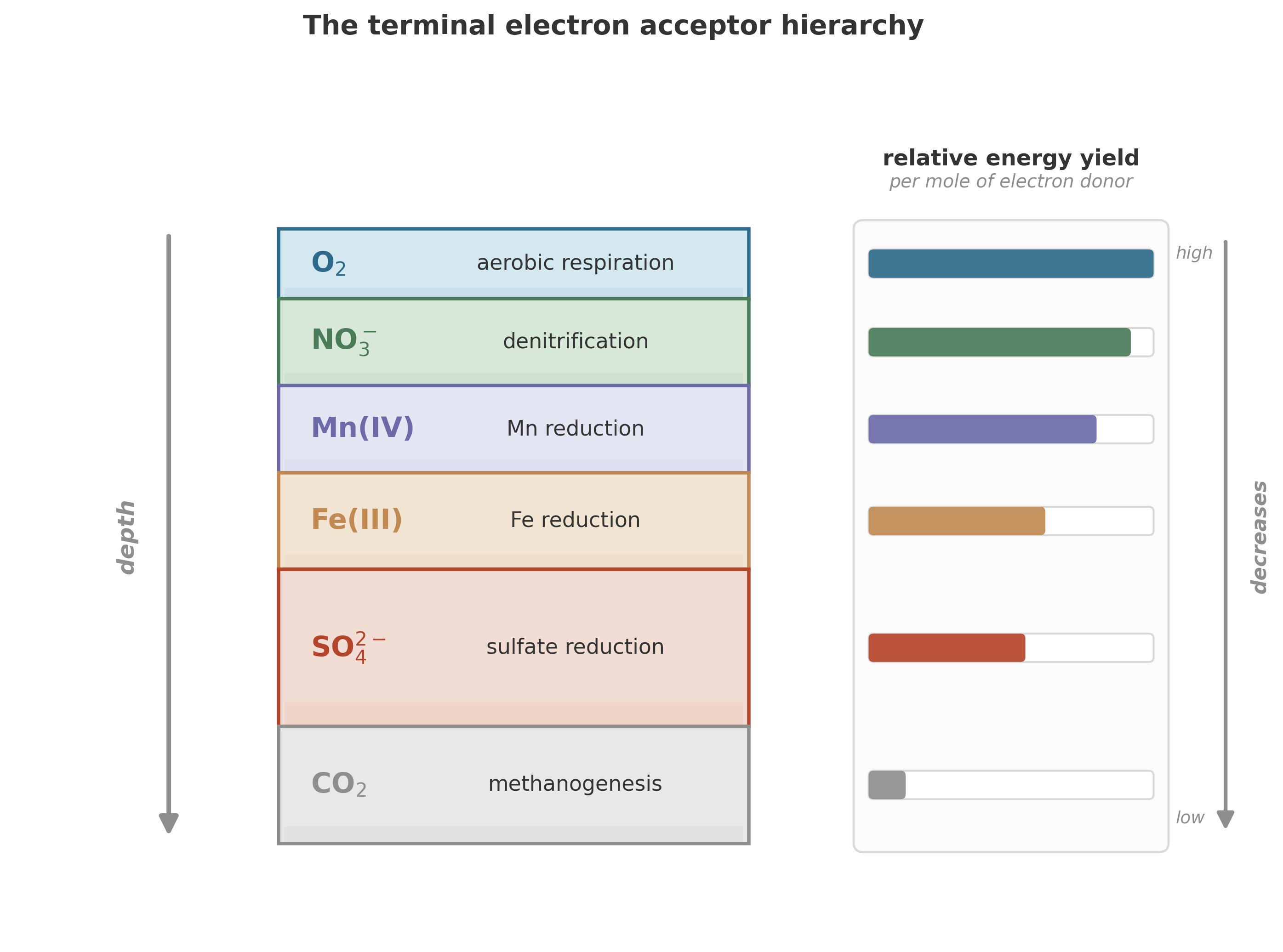
Each acceptor supports a distinct metabolic community: aerobic respirers, denitrifiers, manganese reducers, iron reducers, sulfate reducers, methanogens. These are the Terminal Electron Accepting Processes, or TEAPs, and in an idealized system they appear in sequence as the more energetically favorable acceptors are exhausted.12 Iron and sulfate reducers typically conserve four to five times more energy per mole of electron donor than methanogens – a difference that has profound implications for community structure and biomass yields.13
In practice, the deep subsurface is messier. Lovley and Chapelle noted a tendency in geochemistry to treat microorganisms as “black boxes that may facilitate thermodynamically favorable reactions” – as if the bugs are just catalysts that speed up whatever chemistry the Gibbs energy landscape demands.14 This shorthand works surprisingly often, but it fails in important cases.
The reason is that thermodynamic favorability is necessary but not sufficient. A reaction can be favorable on paper and still not happen because no organism present carries the right enzymes. A reaction can be favorable and fast in a beaker but starved in a pore because transport cannot supply reactants. As Lovley and Chapelle put it: “It is becoming increasingly apparent that even in ancient, relatively nondynamic subsurface environments, simplified nonbiological models do not accurately describe important geochemical processes”.15
The practical consequence is stark: “Most redox reactions do not take place spontaneously but require microorganisms to catalyze them”.16 In the deep subsurface, the biology is not a detail layered on top of the chemistry. The biology is the chemistry, or at least the part of it that actually happens on observable timescales.
10.4 Respiration in the deep
The rate expressions from Chapter 8 – dual-Monod kinetics throttled by both electron donor and acceptor – apply here without modification.1718 What changes is the context.
In shallow, oxygenated environments, aerobic respiration dominates so thoroughly that it accounts for 90–95 percent of all degraded organic carbon.19 But the deep subsurface is almost never oxygenated. In anoxic, nitrate-depleted settings, a division of labor emerges: fermentative microorganisms first break complex organic molecules into simpler ones – acetate, formate, hydrogen – and then respiring bacteria use those simpler compounds as electron donors, passing the electrons to whatever terminal acceptor remains.20 The fermenters and the respirers are partners, not competitors, linked by the small molecules that one produces and the other consumes.
No single organism can do everything. That constraint – the inability of any one species to completely oxidize complex organic matter using a given terminal electron acceptor – is what forces the community to be a community. Even in the Mponeng fracture, where D. audaxviator dominates, those 25 other species are not bystanders. They fill niches that the brave wanderer cannot. D. audaxviator is self-sufficient for its own metabolism – but the fracture ecosystem as a whole runs on a broader set of reactions than any single genome encodes.
10.5 When the electrons move directly
Not every partnership in the subsurface is mediated by a diffusible molecule like hydrogen or acetate. In some communities, the electrons themselves are exchanged directly.
Electromicrobiology studies that exchange. Geobacter and related lineages can transfer electrons to iron and manganese minerals outside the cell, using conductive pili and cytochromes to push respiration beyond the cell membrane.21 In mixed communities, that capacity can become a social technology. Rather than releasing hydrogen for a partner to consume, one organism can pass electrons directly to another – a process called direct interspecies electron transfer, or DIET.22
DIET extends the syntrophic logic from Chapters 7 and 8 into literal electrical contact. One organism’s waste is still another’s fuel, but the handoff can be a current rather than a molecule diffusing through porewater. In sedimentary environments the same principle appears at larger scales in cable bacteria, which link sulfide oxidation at depth to oxygen reduction near the surface by moving electrons across centimeter distances. The old redox ladder is still there. More wires connect it than we once knew.
10.6 Life at the thermodynamic edge
The deep subsurface pushes microbial life to its energetic limits. How slow can metabolism get before it ceases to be metabolism?
The answer is extraordinarily slow. Douglas LaRowe and Jan Amend compiled data on microbial turnover times across a range of natural settings and found that in aquifers, sedimentary rocks, marine sediments, and ice cores, biomass turnover times can exceed 1,000 years.23 In Antarctic photosynthetic communities – admittedly a surface environment, but one where conditions are extreme – biomass turnover times reach up to 19,000 years.
Consider what that means. A community that turns over its biomass once every thousand years is not dead – it is metabolically active, on aggregate, but so slowly that its existence plays out on a geological timescale. Whether individual cells are continuously active at vanishing rates or cycling between dormancy and rare bursts of activity remains an open question.
The range of metabolic rates across Earth’s biosphere is staggering. LaRowe and Amend found that catabolic rates vary over twelve orders of magnitude, from approximately \(6 \times 10^{-9}\) to \(6.66 \times 10^{3}\) nmol cm\(^{-3}\) day\(^{-1}\).24 Twelve orders of magnitude. The fastest microbial communities metabolize a trillion times faster than the slowest. And yet the slowest are still alive.
This raises a fundamental question about maintenance energy – the minimum energy flux a cell needs just to stay alive without growing. In laboratory cultures, maintenance energy can be measured: you starve a culture, track its decline, and calculate the energy cost of keeping the lights on. But in deep subsurface settings, per-cell energy fluxes are “several orders of magnitude lower than maintenance energies predicted from laboratory cultures”.25
Either the cells are dying and being replaced by slow turnover – possible, but hard to reconcile with such low energy fluxes – or our laboratory-derived maintenance estimates are wrong for these conditions. LaRowe and Amend argue for the latter: maintenance energy is not a constant. It depends on growth conditions, temperature, community structure, and the specific stresses a cell faces. It should be treated as a variable, not a parameter.26
The implication reshapes how we model deep life. A cell in a laboratory flask, bathed in rich media at 37 degrees, has a “maintenance bill” that includes the cost of dealing with rapid environmental fluctuations, repairing damage from reactive oxygen species, and competing with neighbors. A cell in a fracture at 2.8 kilometers depth, in stable, anoxic water that changes on geological timescales, has shed most of those costs. It has not optimized for speed or yield. It has settled into a metabolic strategy that covers its costs under those constraints.
This is the satisficing principle as I use the term in this book. Simon coined it for bounded choice, not for microbes.27 Ecologists later used the concept against strict optimal-foraging models, and Carmel and Ben-Haim found that a robust-satisficing model matched much of that field literature better than optimization did.28 Brennan and Lo then showed, in a formal evolutionary model, that selection can preserve bounded strategies when information and computation carry costs.29 I am extending that vocabulary to microbial communities.
D. audaxviator does not maximize anything. It persists. It runs sulfate reduction with hydrogen not because that reaction yields the most energy per electron, but because it is the reaction its enzymes can catalyze with the substrates its environment provides. The “choice” is not a choice at all. Thermodynamic possibility meets enzymatic capability, and genome erosion strips away the unused alternatives. What remains is the toolkit that covers the cost.
The genome also contains surprises: genes for flagellar motility, chemotaxis, and sporulation – capabilities with no obvious role in a sealed fracture. Whether these genes are maintained by cryptic selection, retained by chance, or simply not yet lost is unclear. But their presence is a reminder that even a minimal genome can encode more than its current environment demands.
10.7 Competing or cooperating?
One of the persistent questions in deep subsurface microbiology is whether organisms in these communities are competing for scarce resources or somehow cooperating to optimize the overall energy harvest. The answer matters for modeling, because competition and cooperation lead to different predictions about which organisms persist and at what rates.
Craig Bethke and colleagues examined this question through the lens of the thermodynamic ladder.30 They noted an apparent paradox: iron reducers and sulfate reducers conserve four to five times more energy in their ATP pools per mole of electron donor consumed than methanogens do. If competition were purely about energy yield, methanogens should be consistently outcompeted wherever iron or sulfate is available. Yet in many natural environments, all three groups coexist, sometimes operating at similar overall rates.
One possible resolution is that the organisms are not simply maximizing their own energy harvest. Perhaps the community as a whole tends toward a state that maximizes the total usable energy extracted from all available reactions – a kind of collective optimization.31 Under this view, the community composition is not determined solely by pairwise competition but by a global optimization problem: given the available electron donors and acceptors, what combination of metabolisms extracts the most energy?
The data in this book fit a third possibility: neither individual optimization nor collective optimization, but satisficing. Each organism runs the metabolism its enzymes permit, at the rate the local concentrations support, without reference to any global objective. The community structure that results is not optimal in any formal sense; it is viable. Every guild covers its maintenance costs. No guild is excluded unless its reaction is thermodynamically impossible under local conditions. The coexistence of iron reducers, sulfate reducers, and methanogens in the same aquifer is not paradoxical under this view. It is expected: all three can cover costs, so all three persist. The boundaries are fuzzy because the constraints are fuzzy.
This is an active area of research, and the models are not yet settled. Critics of satisficing make a fair charge: once you price search and information costs into the objective function, you may have optimization again under another name.32 Microbial communities give that critique less force because no organism surveys the whole landscape and no shared objective ties unrelated lineages into one maximization problem. The test stays empirical. If the framework cannot explain fuzzy coexistence, field rates, and persistent low-yield metabolisms better than the optimization stories do, it does not deserve the name.
10.8 Growth, decay, and the meaning of yield
To connect microbial energetics to quantitative models, we need an equation for biomass:
\[ \frac{d[B]}{dt} = Y \cdot R_{\text{resp}} - \mu_{\text{dec}} \cdot [B] \]
Biomass grows in proportion to the respiration rate (scaled by the yield coefficient \(Y\)) and decays at a rate proportional to the current biomass (scaled by the decay constant \(\mu_{\text{dec}}\)).3334
The yield coefficient \(Y\) – the fraction of catabolic energy converted into new biomass – is not a constant. It scales with the available Gibbs energy, but shallowly: even large changes in energy produce only modest changes in yield, because biosynthesis has irreducible costs.35 Theoretical frameworks derive yield from thermodynamic first principles;3637 empirical approaches fit it to data across metabolic types.38
But in the deep subsurface, growth is only half the story. Much of the biomass at any given time may be dormant – alive but metabolically inactive. Models that explicitly track dormant and active cell fractions show that the transition between states can dramatically affect community dynamics and apparent geochemical rates.39 Cells do not respond instantaneously to environmental changes; there is a lag phase between perturbation and metabolic response.40 For stable deep subsurface settings, quasi-steady-state assumptions may hold. For perturbed systems, they do not.
The honest summary: yield, growth rate, and maintenance energy are not constants. They are functions of thermodynamics, environment, and history.
10.10 What the brave wanderer teaches
Return, for a moment, to the Mponeng fracture. A single species, in water sealed from the surface for millions of years, in rock billions of years old, at 60 degrees Celsius and 2.8 kilometers down. No sunlight, no organic rain, no seasonal cycle. Just hydrogen from radiolysis, sulfate from ancient inclusions, and the patient machinery of a genome honed for exactly these conditions.
Desulforudis audaxviator is, in a sense, the purest test of the non-equilibrium trick we introduced at the beginning of this book. It maintains its internal order by harvesting the thin chemical gradients that geology provides, independent of sunlight or photosynthetic products. Its existence shows that the minimum requirements for life are modest: a thermodynamic gradient, however small; a catalytic machinery, however slow; and time.
The mathematics of this chapter – the Monod kinetics, the yield coefficients, the diagenetic equations – are not decorations. They are the tools that let us ask quantitative questions about this alien world. How fast can D. audaxviator grow on the hydrogen flux available? What yield does its sulfate reduction support? How does the community partition the available energy? What happens when the hydrogen flux changes on geological timescales?
These are answerable questions. The models exist. The parameters are being measured. And the answers, when they come, will tell us something profound not just about life in the deep Earth, but about life anywhere that chemistry and thermodynamics permit it – including, perhaps, the subsurface oceans of Europa or the ancient aquifers of Mars.
The brave wanderer descended into the dark and found a way to live there. The equations are our way of following it down.
10.11 Takeaway
- The deep biosphere hosts microbial communities that survive without any connection to photosynthesis, powered instead by geological energy sources like radiolysis and water-rock reactions.
- “Deep” is defined by hydrological isolation, not depth: intermediate and regional flow systems where surface inputs are negligible.
- The terminal electron acceptor hierarchy governs energy metabolism in the subsurface, but biology is not a passive catalyst – organisms determine which thermodynamically favorable reactions actually occur.
- Electromicrobiology extends syntrophy beyond shared metabolites: some subsurface communities exchange electrons directly through minerals, pili, or conductive filaments.
- Life at the thermodynamic edge operates over twelve orders of magnitude in metabolic rate, with turnover times exceeding thousands of years and maintenance energies far below laboratory predictions.
- Quantitative models (dual-Monod kinetics, biomass growth-decay equations, yield coefficients) connect the biology to measurable geochemical processes – but parameters like yield and maintenance energy must be treated as variables, not constants.
Li-Hung Lin et al., “Long-Term Sustainability of a High-Energy, Low-Diversity Crustal Biome,” Science 314 (2006): 479–482. (Lin et al. 2006)↩︎
Dylan Chivian et al., “Environmental Genomics Reveals a Single-Species Ecosystem Deep Within Earth,” Science 322 (2008): 275–278. (Chivian et al. 2008)↩︎
Li-Hung Lin et al., “Long-Term Sustainability of a High-Energy, Low-Diversity Crustal Biome,” Science 314 (2006): 479–482. (Lin et al. 2006)↩︎
Dylan Chivian et al., “Environmental Genomics Reveals a Single-Species Ecosystem Deep Within Earth,” Science 322 (2008): 275–278. (Chivian et al. 2008)↩︎
Dylan Chivian et al., “Environmental Genomics Reveals a Single-Species Ecosystem Deep Within Earth,” Science 322 (2008): 275–278. (Chivian et al. 2008)↩︎
Li-Hung Lin et al., “Long-Term Sustainability of a High-Energy, Low-Diversity Crustal Biome,” Science 314 (2006): 479–482. (Lin et al. 2006)↩︎
George Westmeijer et al., “Candidatus Desulforudis audaxviator dominates a 975 m deep groundwater community in central Sweden,” Communications Biology 7 (2024): 1332. A modern deep-groundwater study showing that D. audaxviator is not restricted to the original South African site. (Westmeijer et al. 2024)↩︎
Derek R. Lovley and Francis H. Chapelle, “Deep Subsurface Microbial Processes,” Reviews of Geophysics 33 (1995): 365–381. (Lovley and Chapelle 1995)↩︎
Derek R. Lovley and Francis H. Chapelle, “Deep Subsurface Microbial Processes,” Reviews of Geophysics 33 (1995): 365–381. (Lovley and Chapelle 1995)↩︎
Derek R. Lovley and Francis H. Chapelle, “Deep Subsurface Microbial Processes,” Reviews of Geophysics 33 (1995): 365–381. (Lovley and Chapelle 1995)↩︎
Serpentinization – the hydration of ultramafic rocks – produces molecular hydrogen abiotically and has been recognized as a key energy source for deep subsurface chemosynthetic ecosystems. (Lovley and Chapelle 1995)↩︎
Derek R. Lovley and Francis H. Chapelle, “Deep Subsurface Microbial Processes,” Reviews of Geophysics 33 (1995): 365–381. (Lovley and Chapelle 1995)↩︎
Craig M. Bethke et al., “The thermodynamic ladder in geomicrobiology,” American Journal of Science 311 (2011): 183–210. (Bethke et al. 2011)↩︎
Derek R. Lovley and Francis H. Chapelle, “Deep Subsurface Microbial Processes,” Reviews of Geophysics 33 (1995): 365–381. (Lovley and Chapelle 1995)↩︎
Derek R. Lovley and Francis H. Chapelle, “Deep Subsurface Microbial Processes,” Reviews of Geophysics 33 (1995): 365–381. (Lovley and Chapelle 1995)↩︎
Derek R. Lovley and Francis H. Chapelle, “Deep Subsurface Microbial Processes,” Reviews of Geophysics 33 (1995): 365–381. (Lovley and Chapelle 1995)↩︎
Qusheng Jin and Craig M. Bethke, “Predicting the Rate of Microbial Respiration in Geochemical Environments,” Geochimica et Cosmochimica Acta 69 (2005): 1133–1143. (Jin and Bethke 2005)↩︎
Martin Thullner, Pierre Regnier, and Philippe Van Cappellen, “Modeling Microbially Induced Carbon Degradation in Redox-Stratified Subsurface Environments: Concepts and Open Questions,” Geomicrobiology Journal 24 (2007): 139–155. (Thullner et al. 2007)↩︎
C. Rabouille and J.-F. Gaillard, “A coupled model representing the deep-sea organic carbon mineralization and oxygen consumption in surficial sediments,” Journal of Geophysical Research 96 (1991): 2761–2776. (Rabouille and Gaillard 1991)↩︎
Derek R. Lovley and Francis H. Chapelle, “Deep Subsurface Microbial Processes,” Reviews of Geophysics 33 (1995): 365–381. (Lovley and Chapelle 1995)↩︎
Alexandra-Elena Rotaru et al., “Direct interspecies electron transfer between Geobacter metallireducens and Methanosarcina barkeri,” Applied and Environmental Microbiology 80 (2014): 4599–4605. A key experimental demonstration of DIET between a metal-reducing bacterium and a methanogen. (Rotaru et al. 2014)↩︎
Alexandra-Elena Rotaru et al., “Direct interspecies electron transfer between Geobacter metallireducens and Methanosarcina barkeri,” Applied and Environmental Microbiology 80 (2014): 4599–4605. A key experimental demonstration of DIET between a metal-reducing bacterium and a methanogen. (Rotaru et al. 2014)↩︎
Douglas E. LaRowe and Jan P. Amend, “Catabolic rates, population sizes and doubling/replacement times of microorganisms in natural settings,” American Journal of Science 315 (2015): 167–203. Comprehensive compilation of metabolic rates spanning twelve orders of magnitude across Earth’s biosphere. (LaRowe and Amend 2015)↩︎
Douglas E. LaRowe and Jan P. Amend, “Catabolic rates, population sizes and doubling/replacement times of microorganisms in natural settings,” American Journal of Science 315 (2015): 167–203. Comprehensive compilation of metabolic rates spanning twelve orders of magnitude across Earth’s biosphere. (LaRowe and Amend 2015)↩︎
Douglas E. LaRowe and Jan P. Amend, “Catabolic rates, population sizes and doubling/replacement times of microorganisms in natural settings,” American Journal of Science 315 (2015): 167–203. Comprehensive compilation of metabolic rates spanning twelve orders of magnitude across Earth’s biosphere. (LaRowe and Amend 2015)↩︎
Douglas E. LaRowe and Jan P. Amend, “Catabolic rates, population sizes and doubling/replacement times of microorganisms in natural settings,” American Journal of Science 315 (2015): 167–203. Comprehensive compilation of metabolic rates spanning twelve orders of magnitude across Earth’s biosphere. (LaRowe and Amend 2015)↩︎
Herbert A. Simon, “Rational Choice and the Structure of the Environment,” Psychological Review 63 (1956): 129–138. Simon introduced satisficing for bounded decision-making under real limits. (Simon 1956)↩︎
Yohay Carmel and Yakov Ben-Haim, “Info-gap robust-satisficing model of foraging behavior: do foragers optimize or satisfice?,” The American Naturalist 166 (2005). Carmel and Ben-Haim tested robust satisficing against optimal foraging predictions across field studies and found stronger support for the satisficing model. (Carmel and Ben-Haim 2005)↩︎
Thomas J. Brennan and Andrew W. Lo, “An evolutionary model of bounded rationality and intelligence,” PLOS ONE 7 (2012): e50310. Brennan and Lo show how bounded strategies can persist under selection when information and computation carry costs. (Brennan and Lo 2012)↩︎
Craig M. Bethke et al., “The thermodynamic ladder in geomicrobiology,” American Journal of Science 311 (2011): 183–210. (Bethke et al. 2011)↩︎
Craig M. Bethke et al., “The thermodynamic ladder in geomicrobiology,” American Journal of Science 311 (2011): 183–210. (Bethke et al. 2011)↩︎
Werner Callebaut, “Herbert Simon’s silent revolution,” Biological Theory 2 (2007): 76–86. Callebaut reviews the attempt to fold bounded rationality back into optimization and argues that the reduction misses what Simon was trying to explain. (Callebaut 2007)↩︎
Martin Thullner, Pierre Regnier, and Philippe Van Cappellen, “Modeling Microbially Induced Carbon Degradation in Redox-Stratified Subsurface Environments: Concepts and Open Questions,” Geomicrobiology Journal 24 (2007): 139–155. (Thullner et al. 2007)↩︎
A. W. Dale et al., “Pathways and regulation of carbon, sulfur and energy transfer in marine sediments overlying methane gas hydrates on the Opouawe Bank (New Zealand),” Geochimica et Cosmochimica Acta 74 (2010): 5763–5784. (Dale et al. 2010)↩︎
Douglas E. LaRowe and Philippe Van Cappellen, “Degradation of natural organic matter: A thermodynamic analysis,” Geochimica et Cosmochimica Acta 75 (2011): 2030–2042. Thermodynamic framework for predicting organic matter reactivity and microbial yield. (LaRowe and Van Cappellen 2011)↩︎
Bruce E. Rittmann and Perry L. McCarty, Environmental Biotechnology: Principles and Applications (McGraw-Hill, 2001). (Rittmann and McCarty 2001)↩︎
J. J. Heijnen and J. P. Van Dijken, “In search of a thermodynamic description of biomass yields for the chemotrophic growth of microorganisms,” Biotechnology and Bioengineering 39 (1992): 833–858. (Heijnen and Van Dijken 1992)↩︎
Douglas E. LaRowe and Philippe Van Cappellen, “Degradation of natural organic matter: A thermodynamic analysis,” Geochimica et Cosmochimica Acta 75 (2011): 2030–2042. Thermodynamic framework for predicting organic matter reactivity and microbial yield. (LaRowe and Van Cappellen 2011)↩︎
Konstantin Stolpovsky et al., “Incorporating dormancy in dynamic microbial community models,” Ecological Modelling 222 (2011): 3092–3102. (Stolpovsky et al. 2011)↩︎
Harvey W. Blanch, “Invited Review: Microbial Growth Kinetics,” Biotechnology and Bioengineering 23 (1981): 1691–1722. (Blanch 1981)↩︎
Cara Magnabosco et al., “The biomass and biodiversity of the continental subsurface,” Nature Geoscience 11 (2018): 707–717. (Magnabosco et al. 2018)↩︎